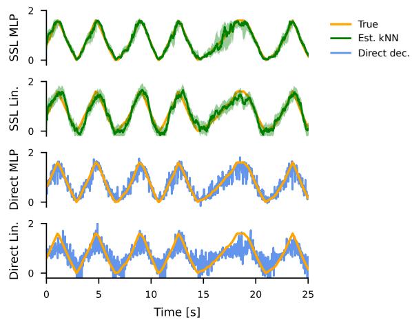
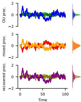
Figure A5Figure A5. Comparison of position prediction through Kalman-based SSL or directly from the data. Kalman-based SSL makes highly accurate predictions with MLP decoder $( R ^ { 2 } = 0 . 9 8 )$ . With a linear decoder prediction becomes worse since at the turning points real position dynamics are not well approximated by a linear model $( R ^ { 2 } = 0 . 8 8$ , similar problem as in Fig. A3). For direct prediction we use the spikes binned in 25ms time windows, which leads to inferior performance of MLP $( R ^ { 2 } = 0 . 8 8 )$ and Linear $( R ^ { 2 } = ) . 5 7 )$ predictors.这张图/表用于判断 Understanding Self-Supervised Learning via Latent 的实验收益来自哪里。重点看替换、消融或跨模型设置下趋势是否一致,而不是只看单个最高分。C Figure 2C Figure 2. Source recovery with LDM in linear ICA. A Linear ICA assumes that the data distribution has independent factors, that can be recovered by aligning them with the correct underlying independent distribution (Cardoso, 2002). B Distributions of pixel intensities in natural images are non-Gaussian (Hyvarinen & Oja ¨ , 1999). In contrast, mixed images are closer to Gaussian, as expected from the central limit theorem. Disentanglement proceeds by learning W to recover an assumed short-tailed distribution (red dashed line). C Also Gaussian sources can be disentangled, which, however, requires more assumptions on the data generating process. Here we recover the outputs of two Ornstein-Uhlenbeck processes assuming known variances and that W is volume preserving (determinant of $| W | = 1 )$ .这张图来自论文 PDF 的结构化抽取。当前用于辅助理解 Understanding Self-Supervised Learning via Latent 的方法或实验,请结合正文精读段落一起看。