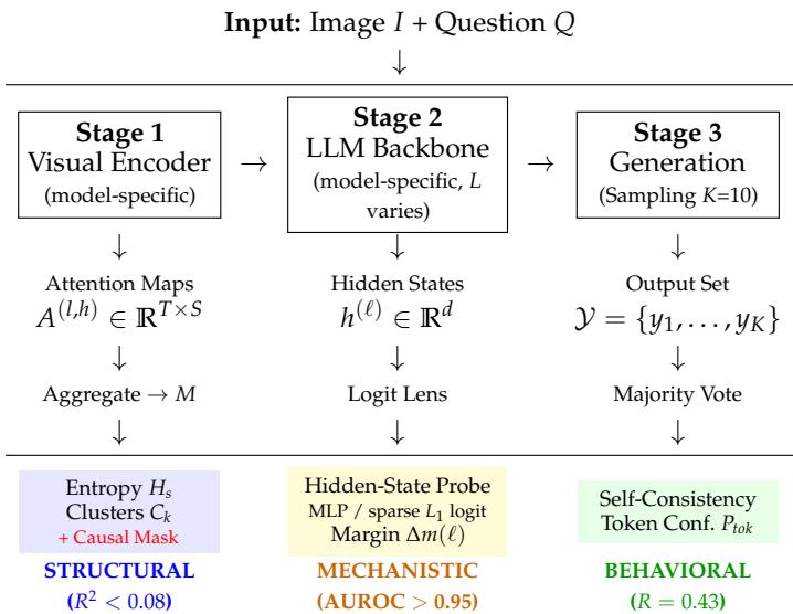
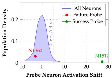
Figureure 1 · : VLM Reliability Probe (VRP) FrameworkFigure 1: VLM Reliability Probe (VRP) Framework. We instrument three computational stages: Stage 1 extracts cross-attention maps from the visual encoder, yielding Structural metrics (entropy $H _ { s } ,$ clusters $C _ { k } ) ;$ we aggregate $A ^ { ( l , h ) }$ by averaging over heads and answertoken positions to form one per-layer spatial vector in $\mathbb { R } ^ { S }$ . Stage 2 probes hidden states via logit lens plus dense MLP and sparse $L _ { 1 } { \mathrm { - l o g i s t i c } }$ probe variants, providing Mechanistic signals; Stage 3 samples $K { = } 1 0$ outputs for Behavioral metrics (self-consistency). Key finding: Structural metrics fail $( R ^ { 2 } < 0 . 0 8 )$ , while Mechanistic probes succeed (AUROC > 0.95). Red indicates causal intervention points.这张图概括 Visuals Lie, Consistency Speaks 的整体方法流程。阅读时先看模块之间传递的训练信号,再看作者如何把目标拆成可优化的子问题。(b) Sparse Circuit: Neuron Distribution Figure 2: Mechanistic analysis of reliability emer(b) Sparse Circuit: Neuron Distribution Figure 2: Mechanistic analysis of reliability emergence. (a) Left panel: Transformer layer index l (x-axis) vs. truth margin $\Delta \mathcal { M } _ { l } \ \mathrm { ( y { - } a x i s ) }$ . Model families display distinct temporal integration profiles: late-emergent $( \mathbf { L L a V } \mathbf { \dot { A } } ,$ , solid blue), earlier-peaking (PaliGemma, dashed red), and cyclical (Qwen2-VL, dotted green). (b) Right panel: Probe neuron activation shift (x-axis) vs. population density (y-axis). The distribution highlights a dense near-zero bulk (most neurons are inactive for truth prediction), alongside sparse, highly predictive outliers (green = success neurons, red = failure neurons) that drive probe discrimination.这张图来自论文 PDF 的结构化抽取。当前用于辅助理解 Visuals Lie, Consistency Speaks 的方法或实验,请结合正文精读段落一起看。