arXiv 新增 + cross-modal on-policy self-distillation · P0 · 2026-06-19

Visual-OPSD：它和通用视觉自监督的关系在于：把昂贵 visual thoughts 的隐式推理能力蒸馏到 text-only student，适合跟 VLM 视觉 latent reasoning 一起看

高相关；详见方法、贡献和实验边界。

Visual-OPSD: Cross-Modal On-Policy Self-Distillation for Efficient Unified Multimodal Reasoning　arXiv 新增 + cross-modal on-policy self-distillation　原文链接

编号2606.18974 优先级P0 类别arXiv 新增 + cross-modal on-policy self-distillation 会议arXiv 新增 + cross-modal on-policy self-distillation 方法把昂贵 visual thoughts 的隐式推理能力蒸馏到 text-only student，适合跟 VLM 视觉 latent reasoning 一起看来源arXiv / OpenReview

先说结论。它和通用视觉自监督的关系在于：把昂贵 visual thoughts 的隐式推理能力蒸馏到 text-only student，适合跟 VLM 视觉 latent reasoning 一起看。高相关；详见方法、贡献和实验边界。

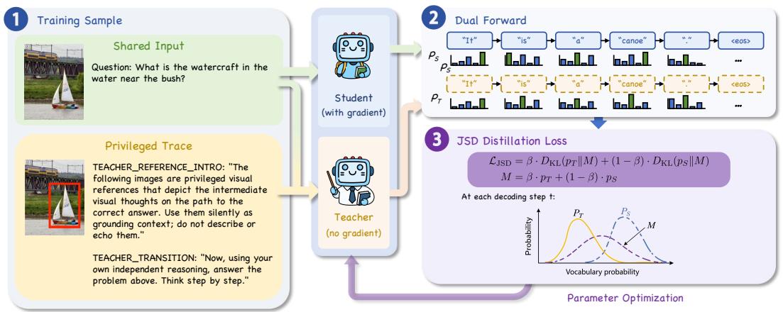
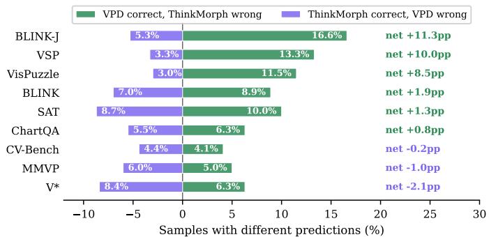
**Figureure 4 · : Overview of Visual-OPSD**Figure 4: Overview of Visual-OPSD. From the same UMM, a student $\pi _ { \theta } ( \cdot | \mathcal { C } _ { S } )$ (gradients on) sees only $[ \mathrm { s y s } , \mathrm { V i T } ( x ) , q ]$ , while an EMA teacher $\pi _ { \bar { \theta } } ( \cdot | \mathcal { C } _ { T } )$ ) (no gradient) additionally receives privileged visual thoughts $( \mathrm { V i T } ( \hat { v } _ { i } ) ) ^ { + }$ +. The student samples $\hat { c } \sim \pi _ { \theta }$ on-policy; both policies rescore the shared completion to yield $p _ { S } ^ { ( t ) } , p _ { T } ^ { ( t ) }$ , optimized by per-token JSD. At inference, the student runs text-only with no VT generation, 14.3× faster, and +3.40pp over the generative teacher.这张图概括 Visual-OPSD 的整体方法流程。阅读时先看模块之间传递的训练信号，再看作者如何把目标拆成可优化的子问题。

**Figureure 5 · : Per-sample win/loss between Visual-OPSD and ThinkMorph**Figure 5: Per-sample win/loss between Visual-OPSD and ThinkMorph. Green: Visual-OPSD correct while ThinkMorph is wrong. Purple: the reverse. Visual-OPSD wins substantially more on VT-useful spatial tasks, while deficits on ThinkMorph-leading benchmarks are small and nearsymmetric.这张图来自论文 PDF 的结构化抽取。当前用于辅助理解 Visual-OPSD 的方法或实验，请结合正文精读段落一起看。

核心问题

它和通用视觉自监督的关系在于：把昂贵 visual thoughts 的隐式推理能力蒸馏到 text-only student，适合跟 VLM 视觉 latent reasoning 一起看。

方法拆解

把昂贵 visual thoughts 的隐式推理能力蒸馏到 text-only student，适合跟 VLM 视觉 latent reasoning 一起看

主要贡献

高相关；详见方法、贡献和实验边界。

实验看点

实验部分建议重点看两类证据：一是作者是否把方法收益和更强数据、更长训练、更大模型区分开；二是跨模型、跨数据或跨任务迁移是否还能保留同样趋势。

局限与读法

这篇论文的结论需要结合任务设置、训练数据规模和消融实验一起看；不要只凭单个指标判断它对通用视觉表征的价值。